


Breaking the Shortest Path Barrier: A Deep Dive into BMSSP
Or how I realized I'm probably not cut out for theoretical computer science

NOTE: This post is a very technical deep dive into the BMSSP algorithm outlined in Breaking the Sorting Barrier for Directed Single-Source Shortest Paths. I recommend reading this post with the paper handy as it’s meant to be used as a resource to learn how the algorithm works. We’re going to go deep into how BMSSP works, what its limitations are, how the actual technical implementation fares against traditional Dijkstra’s, and what the future looks like!
BMSSP
In April, 2025, researchers Ran Duan, Jiayi Mao, Xiao Mao, Xinkai Shu, and Longhui Yin published Breaking the Sorting Barrier for Directed Single-Source Shortest Paths. The paper won a Best Paper Award at STOC for 2025 and claims to have broken the O(n*log(n)) sorting barrier Dijkstra’s algorithm imposes on its frontier. Although the algorithm doesn’t have a specific name yet, it solves a variant of the shortest path problem called the “bounded multi source shortest path” (BMSSP), and so I’ll refer to it as such until we might come up with a different name for it.
What Dijkstra’s algorithm lacks in complexity, BMSSP brings in spades. BMSSP is not an easy algorithm to follow, but the essential idea is based around improving how the frontier in a graph search is generated and avoiding sorting a lot of nodes along the way. Recall the normal single-source shortest paths problem, which goes like:
For a graph G=(V,E) and a node s in V, find the shortest path distances (represented by a function d[v]) from s to all other nodes in G.
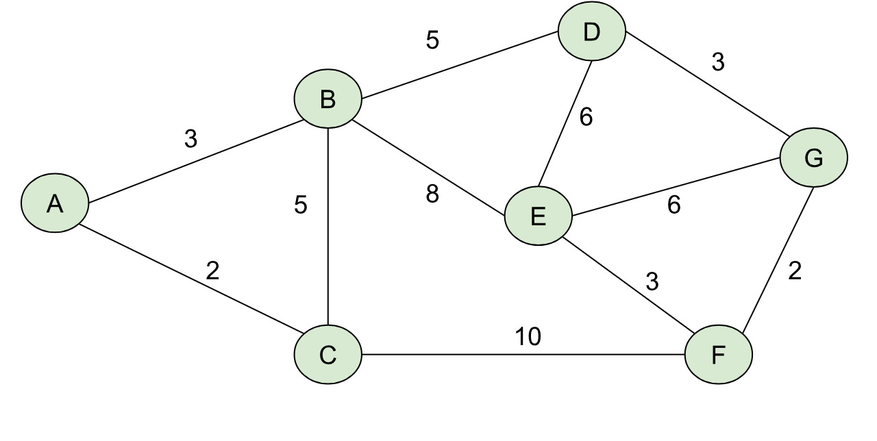
For a graph like the one below:
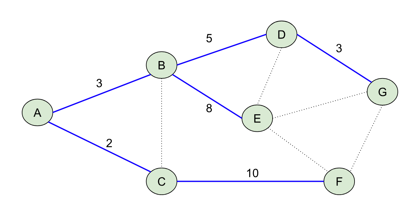
Our shortest path tree rooted at A would like like:
BMSSP generalizes the shortest paths problem to have multiple sources with initial distances and a bound, B:
For a graph G=(V,E), a set of nodes {S} with initial distances, and a real value B, find the shortest path distances d[v] from the nodes in S to all other nodes in G where d[v] < B.
Instead of finding a shortest path tree, BMSSP finds a set of trees rooted at each node in S (a shortest path forest). If we set S to just one node with an initial distance of 0 and we set our bound B to infinity, then BMSSP is equivalent to the shortest paths problem. Make sure this generalization feels clear before proceeding!
BMSSP is clever because it contains a natural way of breaking down the problem into a divide-and-conquer algorithm. To demonstrate this, let’s consider a different graph with some initial distances for nodes (the blue nodes with the numbers inside the circles are our “initial” set):
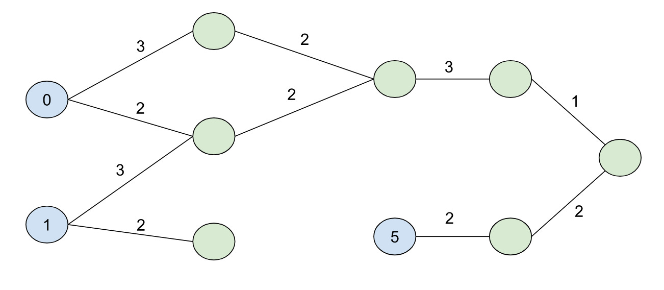
If we set B=9, our shortest path forest would look like:
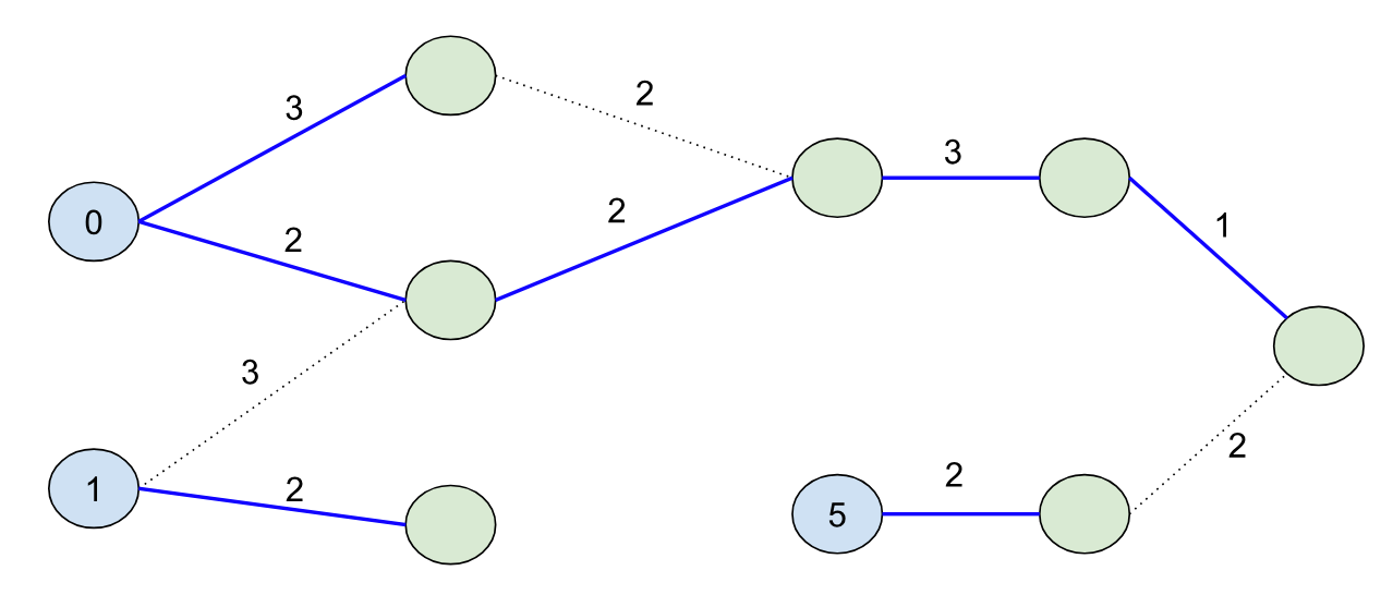
The shortest path forest touches every node in the graph (10 nodes) for this case, but if we set B=4:
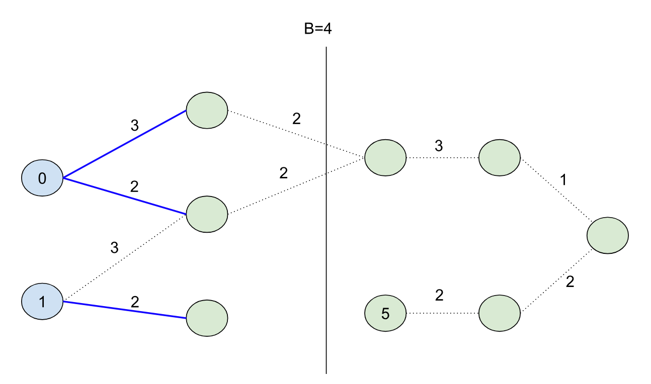
And we’d touch exactly half of the nodes in our search. Note that we didn’t color the node with distance 5 blue this time (because its initial distance 5 is greater than the bound B=4).
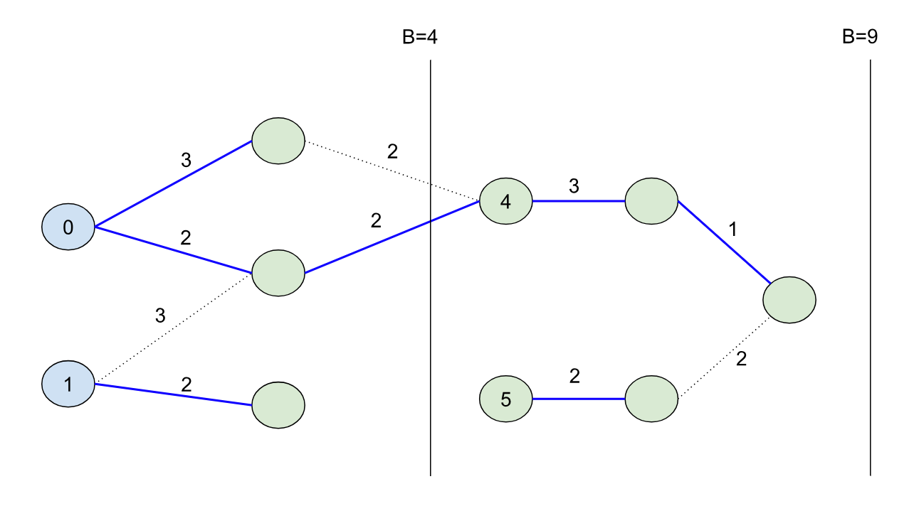
Imagine if we want to solve the original B=9 problem using a kind of “divide-and-conquer” strategy. We can use the shortest path forest created from the B=4 bound because it splits the problem cleanly into two halves: namely, we can characterize the second half of the problem by finding all paths from nodes in our initial set S unioned with all of the nodes that could have come from the first half of the problem. So in other words, we can continue growing the shortest path forest from the first half of the problem into the second half to seed the initial nodes for the second half (in this case the node with initial distance 4):
There are some important takeaways here:
Divide and Conquer: BMSSP naturally breaks up the SSP problem into separate “sub problems” that can be solved separately. Dijkstra’s algorithm can’t be broken up this way because its frontier is entirely dynamic. As Dijkstra’s algorithm searches, a new node it adds can be inserted anywhere in its heap, and so it must maintain a total ordering over its frontier. BMSSP can subdivide using appropriately chosen bounds to guarantee optimality, and if it can keep its frontiers relatively small in each subproblem, it can avoid the overhead of a total sort. The authors of the paper say it well: “Dijkstra’s is to BMSSP as Binary Tree Sort is to Merge Sort.”
Pivots: Note that the node with distance 1 had its shortest path tree end abruptly, while the 0 node’s tree “continued” into the second half of the problem. 0 in this case is called a “pivot” node, and a large part of making BMSSP efficient is to identify these pivot nodes quickly during the search using Bellman-Ford-like updates. When pivots are identified and after the Bellman-Ford updates, we can effectively remove the non-pivot nodes from our search, which keeps the frontier small!
Picking Bounds: In the example above we knew our distances and could select bounds to divide up the problem into perfect halves. The paper does this differently by breaking up the problem into 2t disjoint sets (where t=log2/3(n)), and dynamically finding the bounds as it searches. This selection of t serves as a first hint as to where the strange time complexity is derived from.
Selecting Pivots
From the paper (with some symbols/words changed for clarity):
Suppose at some stage of the algorithm, for every u with d(u) < b, u is complete and we have relaxed all the edges from u. We want to find the true distances to nodes v with d(v) ≥ b. To avoid the Θ(log n) time per node in a priority queue, consider the “frontier” S containing all current nodes v with b ≤ d[v] < B for some bound B (without sorting them). We can see that the shortest path to every incomplete node y with b ≤ d(y) < B must visit some complete node in S. Thus to compute the true distance to every y with b ≤ d(y) < B, it suffices to find the shortest paths from nodes in S and bounded by B.
From the graph above, you can think of this stage as being after we’ve solved the first half (where B= 4). And now our frontier is the node with distance 4 and node with distance 5. The two big things this paragraph is saying are that:
Every incomplete node must visit some complete node in the frontier.
If we find the shortest paths from the nodes in S, we’ve found the true distances to every node in this subproblem.
Additionally, the algorithm states two possible outcomes as a result of running BMSSP:
The BMSSP returns a set of complete nodes, U, and a bound B’=B. This means it found the true distances to all nodes with distance < B successfully.
or BMSSP returns a set of complete nodes, U, whose size has exceeded some parameterized value and a bound B’ < B. This is also called a “partial execution”, and is used to avoid having BMSSP spend too much time processing the nodes of a frontier with a bad boundary value. This is useful because we don’t know in advance what our boundary values ought to be to properly divide up the problem equally!
Part of shrinking the frontier for subsequent subproblems is to only select pivot nodes to seed the next piece of the frontier appropriately. The way we do this is by running k Bellman-Ford “relaxations” over the edges in our current frontier, which constructs a shortest path forest rooted at most |U|/k pivots. This is based on a sort of pigeonhole principle argument: if we return the roots of trees with at least k nodes, then we can’t return more than |U|/k roots and running Bellman Ford k times over the nodes in our set will generate a set of complete nodes that are up to k edges away from a root.
Selecting k appropriately then becomes very valuable as a time-complexity knob. Using k=log1/3(n), the authors are able to make some arguments to bound the worst case complexity elsewhere. For a large enough graph (like 50 million nodes), k is still relatively small (2), so the number of Bellman Ford updates stays pretty small too.
The Block List
One other innovation BMSSP uses is a specialized data structure (a block list) that maintains a kind of “semi” sort over its elements. Effectively it lays out its elements and costs in a flat array of blocks where each block contains an upper bound, but the elements in the block need not be in sorted order. The only requirement is that for two consecutive blocks Bi Bi+1, each of the elements in Bi are less than the elements in Bi+1. Because BMSSP limits the size of each block to an integer parameter, M, it can retain tight time complexity bounds.
The block list allows for prepending batches of elements that we determine are cheaper than our current bound (without any sorting). It also supports pulling the M smallest elements as well as their current upper bound (kind of like a heap pull + peek), without storing the values in a heap1. Without this operation, the block list would not be able to beat the time complexity capabilities of a standard binary heap and so its necessary for the correct implementation of BMSSP.
An Example Run of BMSSP
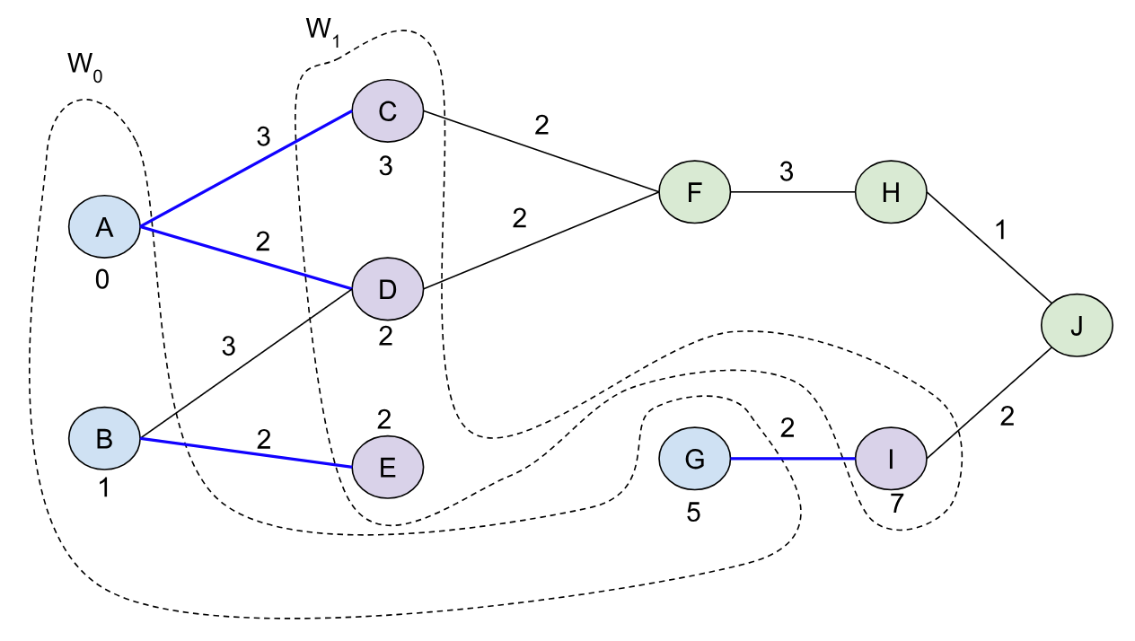
At this point I think it’s worth actually trying to see what BMSSP actually does with the sample graph we had from above. So let’s initialize S = {A, B, G} with B=9 for the graph (I went ahead and named the nodes with letters to differentiate them from their distances more easily):
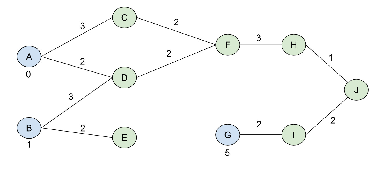
Note we also have the distance function defined for this initial, complete frontier, d[v], where d[A]=0, d[B]=1, and d[G] = 5. d[v] for the other nodes is set to infinity to begin with. We’ll use k=2 and t = 2, which means our “l” levels start from ceil(log(10)/2) = 2 and go down to 02.

l=2
Following the paper, we’ll call: BMSSP(l=2, B=9, S={A, B, G}). As we can see on line 4, our very first item of business is to find the pivots with our current frontier. We do this by expanding out the edges from the pivot and building out “layers” (the Wi values in the algorithm).
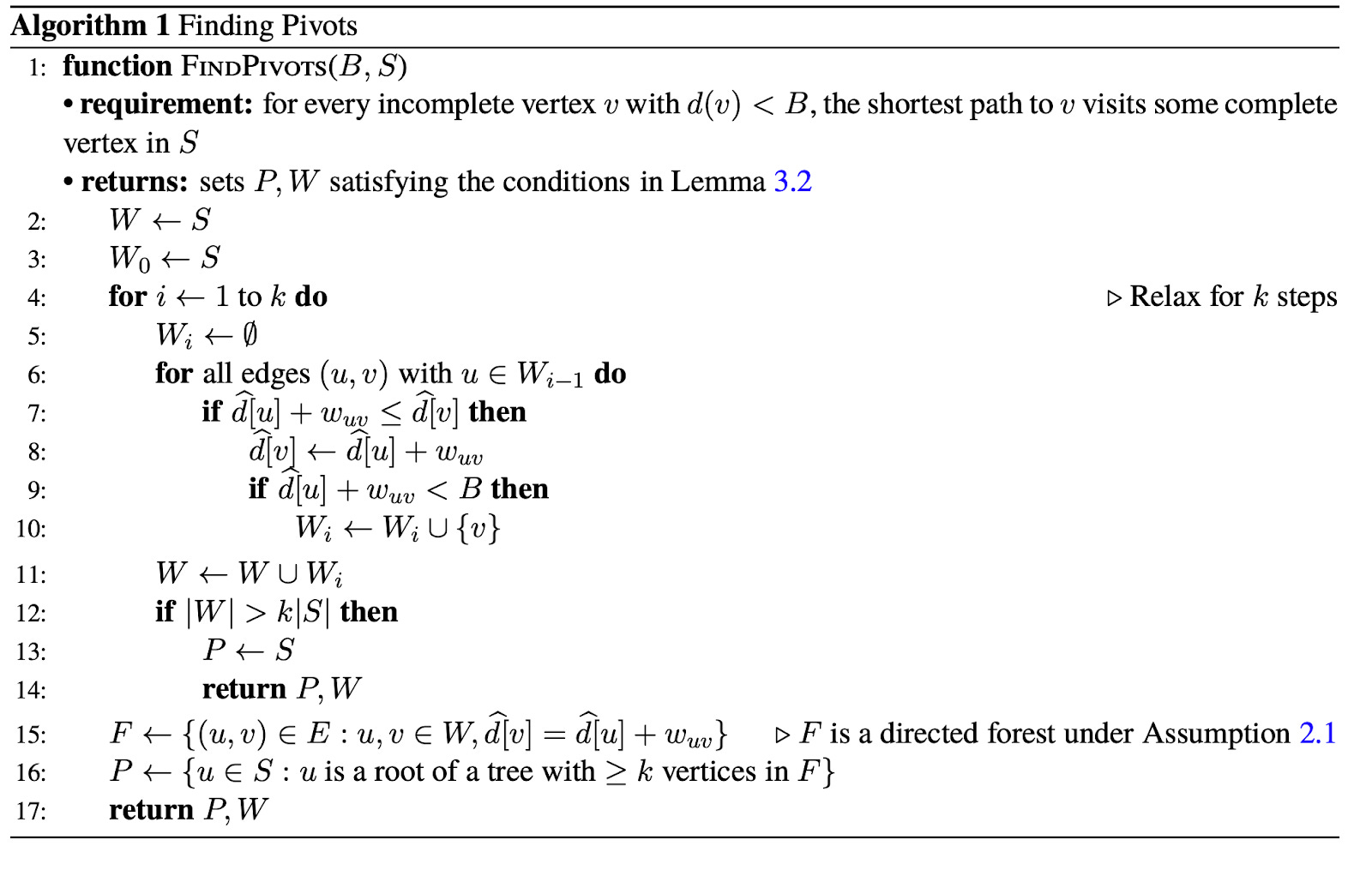
In this case, W0 = {A, B, G} (the initial frontier) and when we explore edges from W0 we’ll add those new nodes to W1, and continue this procedure until we’ve explored more than k * |S| = 2 * 3 = 6 nodes. So our W layers will expand up to W1 before terminating:
At this point we return back the nodes in W0 and W1 (not in order), and the pivots (A, B, G). We initialize our special queue (D) with M=2^((2 - 1) * 2)=4 (line 5 in the algorithm). Then we insert the pivots with their distance costs into D and set the bound B0’=0 (the minimum of these pivot distances). Our queue looks like this at this point:
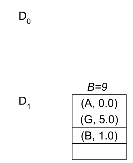
Note that we don’t keep a sorted order and we have up to 4 nodes per block. Right now we’ve inserted the 3 pivots, so we don’t need more than one block.
In the main loop, we pull up to M=4 elements with their upper bound. In this case it’s just the pivots with the bound 9 (line 9). Then we recurse and call BMSSP(l=1, B=9, S={A, B, G}).
l=1
You can check for yourself that this call will result in the same pivots as before, but now we’ll use M=1 blocks for the data structure, and our blocks will look slightly different:
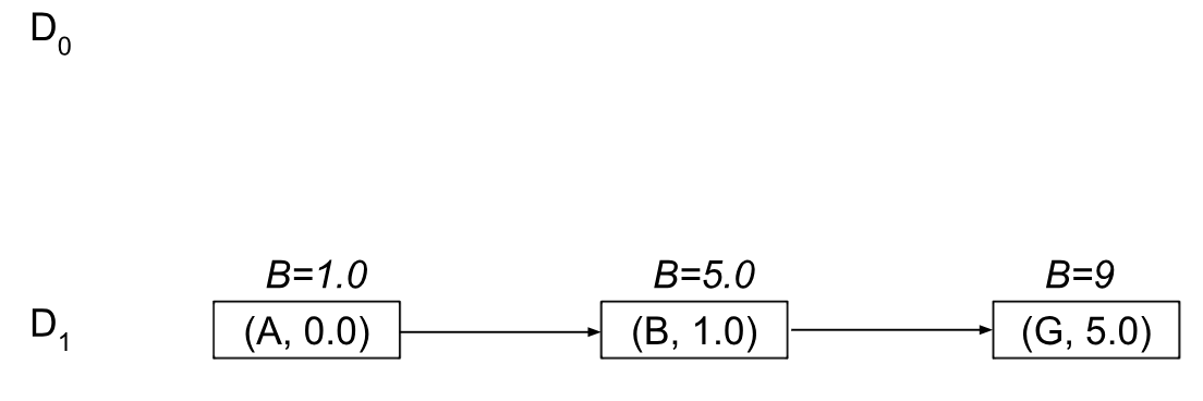
Note that we’ll always eventually get to this kind of “flat” M=1 structure as soon as l=1. This is how the “l” levels partition BMSSP recursively until becoming a single node to run the base case from: (see line 5 in Algorithm 3 to check). So now when we “pull”, we’ll get the node A with a bound of B=1.0 and recurse into BaseCase(B=1, {A}):
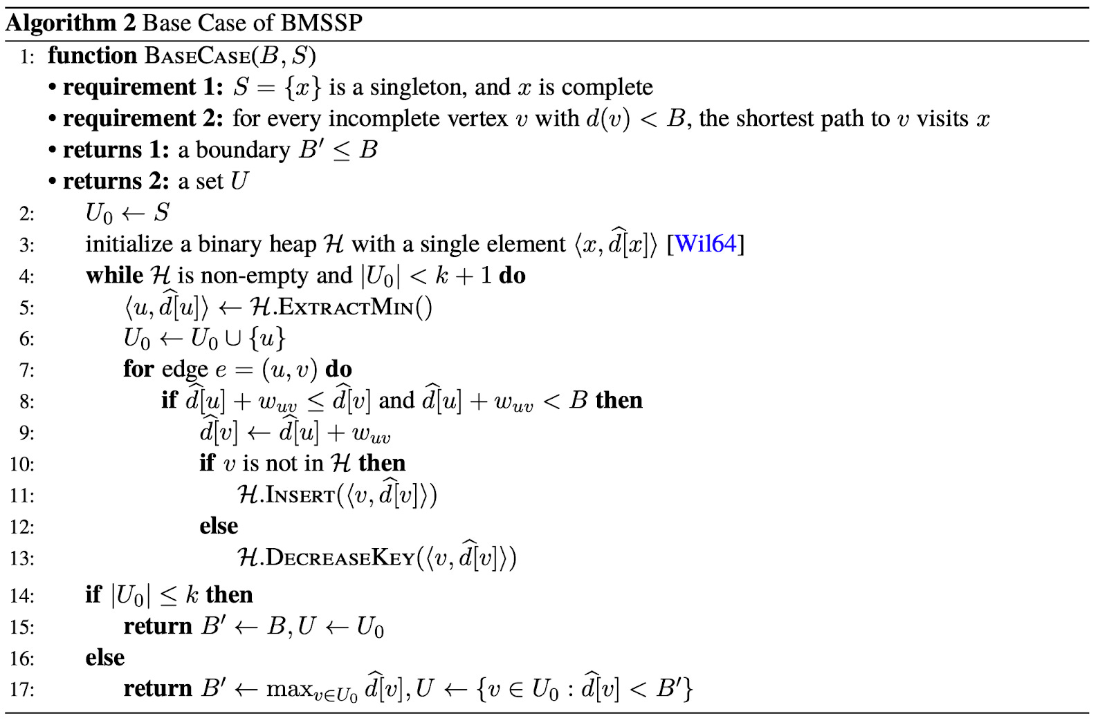
l=0
This part is like a mini-Dijkstra’s algorithm from the single element we pulled. Effectively, we search out until the number of nodes we explore (U0) is of size k + 1. In this case (k=2), this means we’ll close up to 3 nodes. However, because our bound is 1.0, this means we don’t actually close anything beyond the starting node A! So we’ll quickly return at line 15 with the same bound we passed in (B’=1) and the set U={A}. Note that at other times, (like if our bound is too loose), we’ll explore more than k nodes and “shrink” our bound at line 17.
l=1
Once we return back to the upper level of BMSSP, we’ll explore and insert again from A. Inserting the neighbors of A means our data structure will change again to look like the following to accommodate adding C and D.

Note that inserting the new values will “split” blocks, which also update the upper bounds for the nodes appropriately in the structure. We’ll continue this process of pulling and updating our Bi’ boundaries until we exhaust our list of nodes or explore too many. In this case, we stop after exploring {A, B, C, D, E, F, G, H} because our block list gets too large (8 elements long). Recall that this is how BMSSP attempts to partition the problem into equally spaced chunks. In this case it doesn’t do great (e.g. a split of 8 and 2 for 10 nodes is kind of silly), but the idea is to limit BMSSP from doing too much work in any one recursive call.
l=2
After returning, we have an updated boundary B’=7 and set U = {A, B, C, D, E, F, G, H}. We end up adding nodes I, and J into our block list, prepending them into the D0 blocks because their values are now between [7, 9):
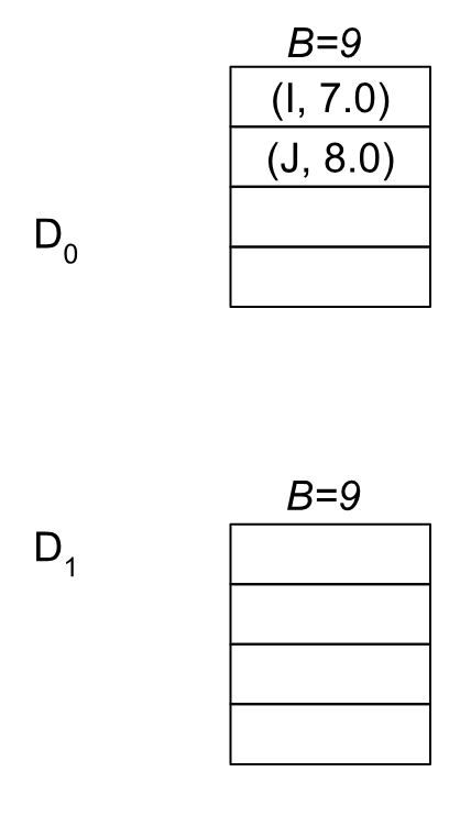
.
After we return back, we’ll call FindPivots with the new frontier {I, J}, and quickly terminate the next BMSSP call. You can see how BMSSP shifts up its the boundary and “seeds” subsequent iteration calls with the results from the previous one. For example in this case it broke the problem into a half which called up to B=7, and then the second half between B=7 and B=9. This is how BMSSP leverages divide and conquer effectively in its structure, although it remains to be seen what, if any, parallelization could be leveraged here.
Results and What Lies Ahead
I’ve implemented BMSSP in Rust alongside Dijkstra’s and run it on some relatively large road networks (e.g. the DC metropolitan area and Northern California). As of right now, my implementation of BMSSP runs roughly 5-7 times slower than Dijkstra’s on these graphs.
This may seem a bit surprising after all of this work, but it’s worth clarifying some things. One big piece to note is that theoretical time complexity gains do not always translate to real world gains. This is why even though a linked list offers O(1) insertion and deletion operations at the head or tail of the list, they fail to beat a double ended queue in the real world due to things like cache locality and optimized memory layouts on real-world architectures.
We should also keep in mind that my implementation of BMSSP is the slowest it will ever be3. It is a representative algorithm, but it’s certainly not optimized as well as it could be. It makes many recursive function calls, relies on suboptimal memory layouts (e.g. non-cache optimized, heap-allocated memory). Compare that for example to the equivalent Dijkstra’s implementation, which runs in one stack frame with a single binary heap.
If we can get BMSSP significantly faster than Dijkstra’s by optimizing it well, I think there are a number of ways to potentially make it very useful:
CRP Preprocessing: In algorithms like CRP, we need to solve many SSP’s to create shortcut edges. BMSSP could be used as a base algorithm to find these shortcut edges and speed up the preprocessing phase.
Extending with A*: BMSSP solves the single source shortest path problem, but more often than not we need just one path to a destination. For these problems we use algorithms like A*, by deprioritizing particularly bad nodes from the search. Because A* can be seen as running Dijkstra’s on a modified graph (e.g. the cost c(u,v) for an edge (u,v) becomes c’(u,v) = c(u,v) - h(u) + h(v)), we can run BMSSP using heuristics and terminate the algorithm once our destination node is closed to find a single path.
Finding Landmarks: Creating strong heuristics for A* using landmark heuristics require running many SSP queries (from one node to all nodes in a network or vice versa). Doing this more quickly makes creating heuristics much cheaper for real-world algorithms.
If you’re interested in seeing and/or contributing to the BMSPP implementation outlined here, you can check out the code at github.com/rap2363/ssps.git. I’m happy to welcome pull requests to improve and benchmark BMSSP against Dijkstra’s. Let’s see how fast we can make BMSSP go!
As I write this I realize there’s probably a way to make the block list very memory-friendly e.g. using a stack implementation instead of a linked list.
Technically we should set k=1 for a graph this size, but that would make for a very lame-looking algorithmic run.
In fact, switching over to using better-performing hash maps in Rust sped it up by nearly 30% from my very first iteration!