
Stochastic Optimization and Dispatching Drivers
Or how I learned to love value functions again

I was looking through my old grad school notes and came across an interesting problem from my stochastic control theory class1. The idea is as follows: you’re managing a queue of packets that you’re trying to send out over some noisy, wireless channel. Every fixed time interval you have a new number of packets arriving, and you have a decision to make over how many packets you want to send out. At every epoch there’s some amount of noise in the channel, which impacts the required power it takes to send out the packets in that time slot (i.e. more noise requires more power). In the problem there are two primary costs we’re minimizing:
Queueing Cost: This is a quadratic function based on the current number of packets in the queue and it roughly captures the average delay per packet (i.e. this being large means we’ve not been sending out packets and are delaying the transmission).
Transmission Cost: This is a cost dependent on both the number of packets we want to send out as well as the wireless channel noise in the current epoch. This cost can be modeled as roughly exponential with respect to the number of packets you’re sending and proportional to the noise in the channel.
The idea is to come up with a control policy that minimizes the long-running average queueing and transmission costs. But as I was mulling it over I realized that this structure (balancing delay against variable service cost) maps surprisingly well to ride share dispatch!
Dispatching Drivers
Instead of sending out packets, suppose we’re a ride share company with a number of drivers at our disposal to service incoming ride requests. There’s some cost for queueing and having riders wait, and there’s also some cost to dispatch drivers (maybe based on current traffic conditions and the ability to pool riders together). As customer requests come in, we have the option to “service” a number of requests by dispatching a number of drivers and we must make a decision of how many requests to service. Similar to the wireless transmission problem, we can model this with two costs to trade off:
Request Storage Cost: Effectively this can be thought of as our average delay for servicing requests and ensures our queue doesn’t stay too full over time. Similar to the packet transmission use case, we let this be a quadratic function to penalize keeping too many requests in the queue (modeling situations where it gets worse and worse to keep riders waiting for a driver to service them).
Dispatch Cost: For the ride share use case, we can model our dispatch cost as stochastic and dependent on an “optimized pooling” value, which represents how costly it currently is to service a number of requests. This cost is proportional to max(1, qt - pt) and models the idea that we can wait until we get a good “pooling” option before dispatching some number of drivers. Crucially, a high pt value means we can service more requests without incurring more cost.
Our service runs for a long period of time, and we want to minimize the average “cost” per dispatch decision (the sum of the long running average queueing cost and dispatch cost). Like before, we want to balance having a small queue (i.e. minimizing request delays) against optimizing how “good” dispatches will be if we wait for a little while. A familiar scenario is when you’re waiting for your Uber or Lyft app to send you a driver (internally your request is enqueued and they’re figuring out which driver to dispatch to you and how to optimize their driver network as a whole).
So the question is, if we have some understanding of what the distribution of requests and pooling costs looks like, can we implement a good policy for dispatching drivers?
Problem Specification
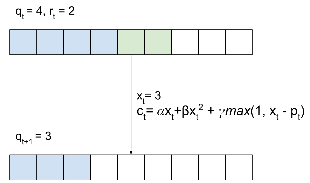
Let’s restate the problem and define our variables and setup clearly before proceeding. At every time epoch (indexed by t), we have the current number of requests in the queue, qt, along with a number of new requests, rt, and a pooling benefit parameter, pt. We assume that rt and pt sample from some known distribution (e.g. rt is the number of requests that come every 15 minutes if we’re indexing time in 15-minute increments). At every t we can pick how many requests we’d like to service, xt. Finally we have some parameter Q, which represents the maximum size of our request queue (to ensure we never accumulate too many requests without servicing them). The evolution of our system can be modeled by:


And we’re minimizing the long running average of a quadratic queueing cost and pooling cost:

To illustrate this more explicitly, I’ve included an example of a state transition of the system with xt=3 (i.e. we choose to service 3 of the rider requests, which incurs some cost ct).
Our goal is to find some policy (i.e. a rule based on the queue size, number of new requests, and pooling costs) that can help us minimize the average dispatch cost.
Finding a Greedy Policy
Let’s start off with a simple policy to get our footing on the problem. In the real world, well-tuned greedy policies can perform quite well for a number of use cases, and it’s a good idea to understand just how suboptimal (or not!) they are in certain cases. I’ll propose a simple, threshold-based policy:
If the number of requests exceeds a threshold, service just enough of them to get us back under the threshold.
Otherwise, service pt requests (or all of the requests if we have less than pt requests in the queue). This takes advantage of the pooling benefit whenever it’s high.
The benefit of such a policy lies namely in its ability to code up and scale, but this policy is limited in that it doesn’t account for or attempt to optimize with respect to the probabilistic distribution of the request arrivals or the pooling costs.
Now that we have a policy, how should we evaluate its utility? The simplest way to do so is to run a simulation! We’ll use the following parameters:


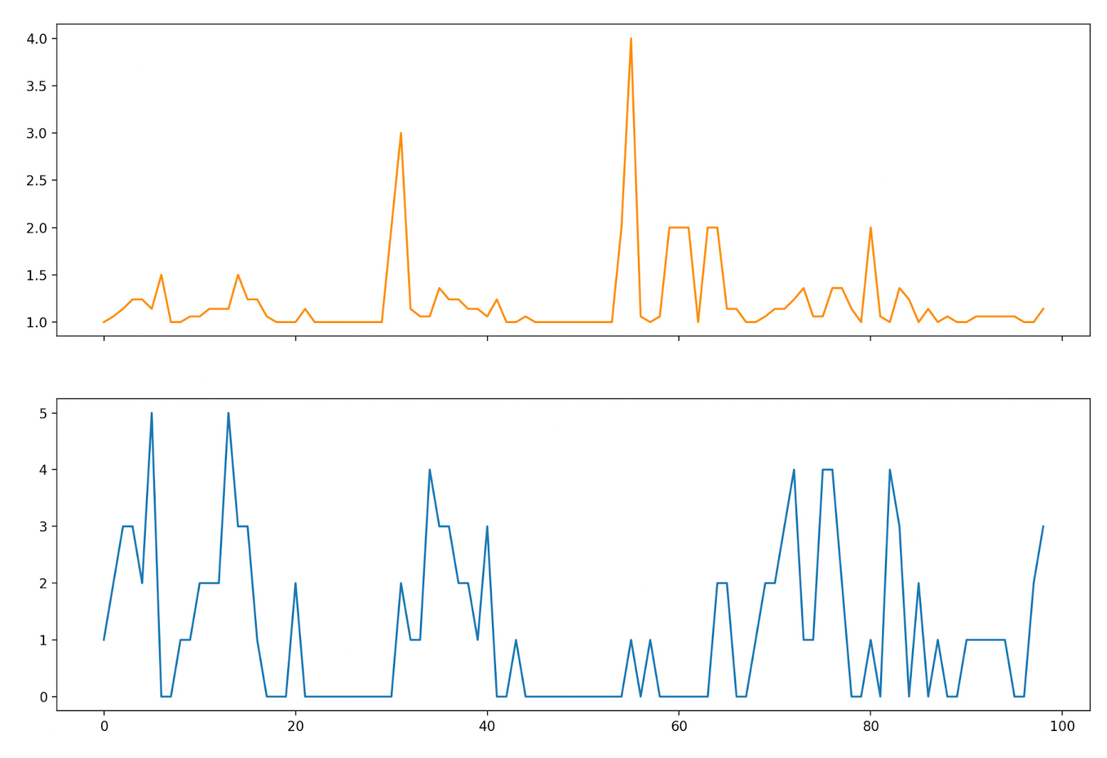
Where rt and pt are independently distributed according to the distributions above (e.g. pt is 5 with probability 0.1). We can simulate how the policy does over 100 time steps (by sampling from the pt and rt distributions and enacting the greedy policy), and then plotting our costs (orange) along with our queue size (blue):
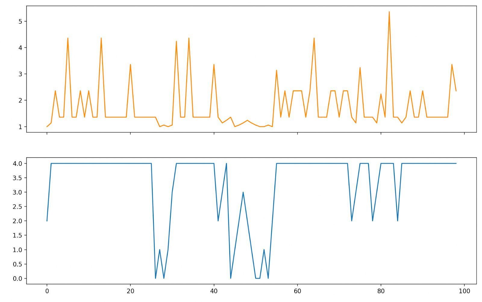
With our thresholding we don’t allow our request queue to exceed a size of 4, and are forced at certain points to service requests at a high cost (resulting in big “cost spikes” at various points in the simulation). Our average cost in running this was 1.75 per time step.
It’s worth noting that our greedy policy does not incorporate any notion of how arrival or pooling benefits are distributed. In other words, it doesn’t “look ahead” to minimize expected cost later down the line. What if we did?
Optimal Control Policy
The next question is, how much better can we do if we incorporate understanding of the distributions into our policy? As it turns out, this is an example of a well-known stochastic process called an MDP (Markov Decision Process), and due to the size of the states, we can generate an optimal control policy relatively quickly through value iteration. Even though our cost functions involve particularly tricky looking non-linearities (like the point-wise max function), we can derive a control policy which will optimally outperform any other greedy policy we could come up with.
Our first step is to outline the value function for this problem. The value function maps the states of the MDP to the expected “cost to go” from that state following some policy. We can model a value function over the state space like so:

However, there’s one slight complication: MDP’s are generally used to solve cost functions whose future costs are discounted by some parameter2. This is important for the value iteration to converge, otherwise in the way we’ve framed it above, we’ll have circular dependencies and costs that will diverge to infinity if we use traditional value iteration.
In this case we can still use value iteration, but we can stop once the differences between our values converge per update. In other words, we can define the update equation like so:

With the defined value denoting the max difference for the kth update:

And our value iteration is complete when this value converges (i.e. 𝛿k → 𝛿*). At this point we have the tools at our disposal to find an optimal control policy for the problem. And like before, we can simulate a sample run using the optimal control policy:
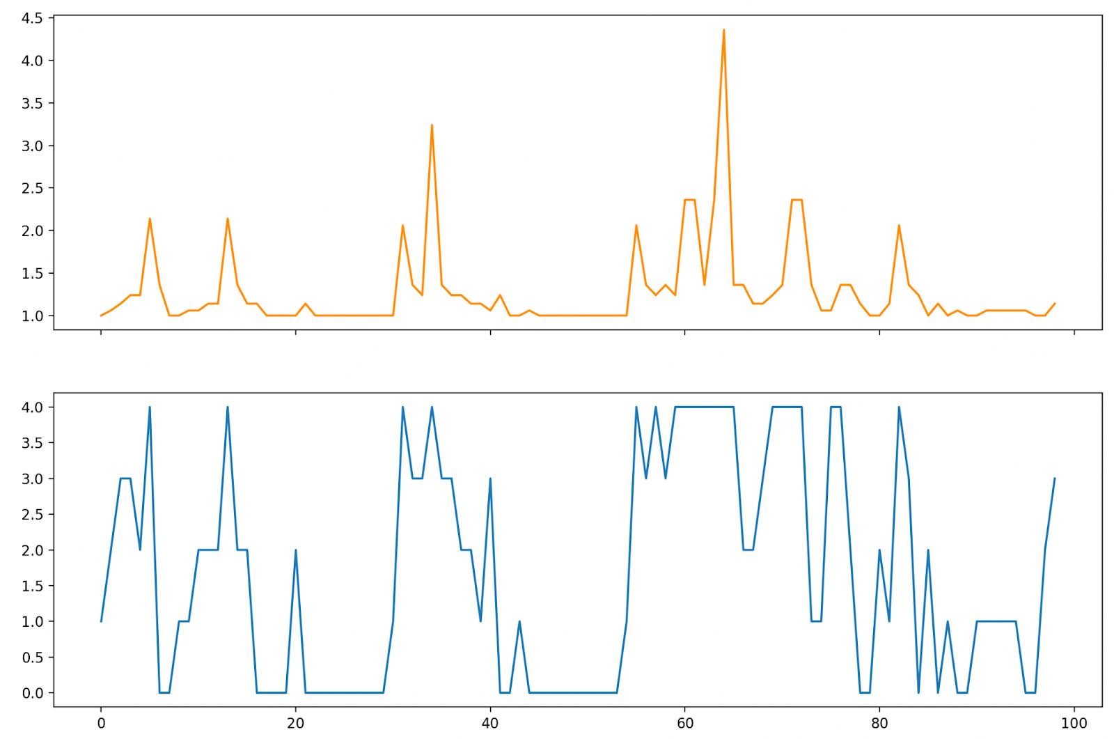
Comparing the costs to those from above, we can see that this results in a significantly better solution (our average cost per time step here is 1.28, roughly a 30% improvement). In our optimal policy we have less “large” spikes, and we don’t keep our queue size at 4 for as long as we did in the greedy policy. We’re able to take advantage of the pooling benefit more regularly and trade off between the queueing and storage costs appropriately.
How Good is Optimal?
Before patting ourselves on the back for the improvements, we should ask how good our control policy truly is. After all, it’s not particularly meaningful to talk about optimal control policies if we don’t have a good benchmark to measure it against. For example, could we have done better if we had a better understanding of the system? What if we could predict with more certainty the actual distributions of pooling costs and arrivals?
We can employ a technique where we build something called a prescient policy. In other words, we create a sequence of sampled values for the pooling costs and arrival rates (just like we did in the Monte Carlo simulations earlier), but now we use those to build a policy that acts as if it knows the entire set of realizations. In other words, we build a policy that can minimize the cost even better because it knows the future.
Even though we can’t actually build something like in the real world, the prescient policy can act as a benchmark or standard by which we measure the performance of our optimal control policy (or any policy for that matter). It’s like a way of zeroing out our comparison scale (e.g. we can ask: how close is our policy’s performance to a perfect one?) and it provides a sort of optimality certificate. For example, if we construct a policy that is within a few percentage points of the prescient policy, it may not be worth investing much more effort in trying to improve the policy. Normally, even constructing a prescient policy can be difficult or near-impossible, but in this particular case we can do so quite easily.
We have a state space with tuples (qt, rt, pt) at each time step and the size of the space is the product of each of the spaces (e.g. for a queue size of 20, 6 possible arrival values, and 4 possible pooling benefit parameters, we have 20 * 6 * 4 = 480 states). If we’re simulating over T time steps, we can think of the equivalent trellis graph where we have 480 states per step, with edges connecting between the layers at t and t+1 according to an action (servicing a number of requests). Visually:
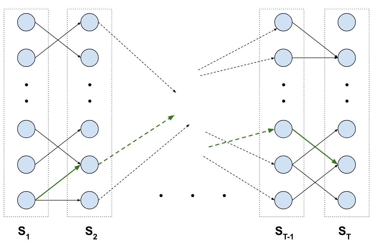
An edge between a state in St to St+1 represents an edge whose weight is equal to to the cost of taking that action (i.e. the queue plus dispatch cost). Our prescient policy is then the shortest path (the green edges) from our starting state at S1 to any of the states in ST. Fortunately, we can run Dijkstra’s on this unrolled graph and obtain the answer (our prescient policy) very easily.
Like before, let’s simulate the prescient policy:
The cost here is lower, but not by that much. In fact, in this run the prescient policy cost is 1.22, roughly a 5% improvement from the optimal policy. Recall that this improvement is from the fact that it knows the exact arrival and pooling parameter patterns and can find the best hypothetical solution.
To me, this relatively small improvement felt a bit surprising, mainly because our optimal policy is only using expected costs3. I find it remarkable that our optimal policy is this close to the absolute upper bound without adding a ton more complexity!
To get a better sense of how these performance improvements looks over longer running averages, we can repeat the Monte Carlo simulation across a number of runs. Here’s what our costs look like using all three policies across 1000 runs:
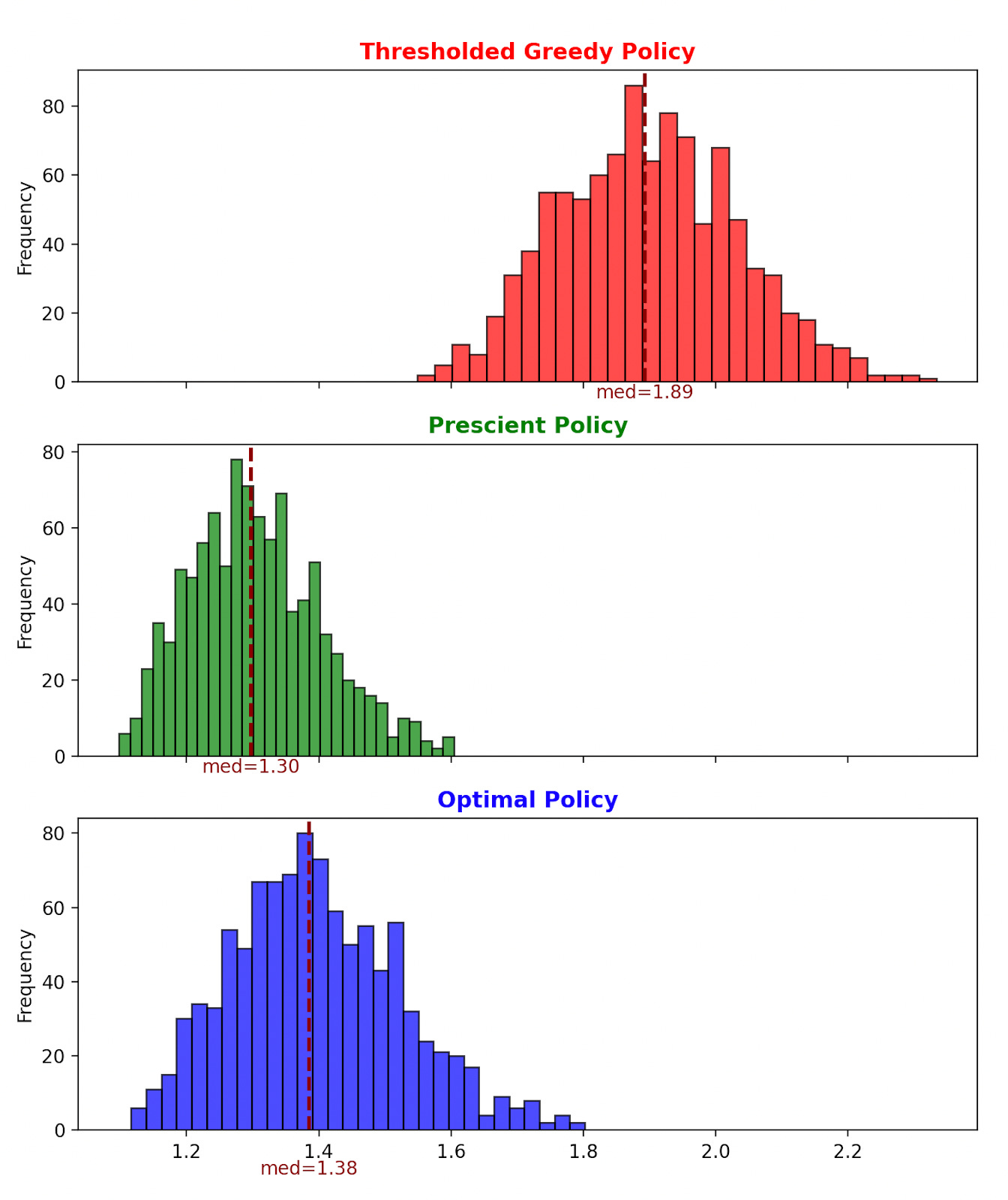
Recall, the best we could do if we knew the future is the green histogram above. By implementing an optimal policy over a greedy one here, we can improve our performance to get significantly closer to the theoretical limit!
What excites me most is how transferable these concepts are. We explored a ride share use case, but stochastic optimization applies generally to many more applications – scheduling drone deliveries, optimizing a financial portfolio, allocating compute, figuring out which bathroom to go to, etc..
If you’re wrestling with your own gnarly technical challenges and want to work with me, please reach out at rohan@rparanjpe.com or visit my website to see what I offer. And if you’d like to try running the code yourself or tweaking with the parameters/logic, you can use this notebook!
That or a process that ends in some a set of terminal nodes with 0 reward.
Actually, our optimal policy is finding the shortest stochastic path through the unrolled graph from earlier. In comparison, the prescient policy was finding the deterministically correct shortest path.