


A New Shortest Path Algorithm
Is Dijkstra's cooked?

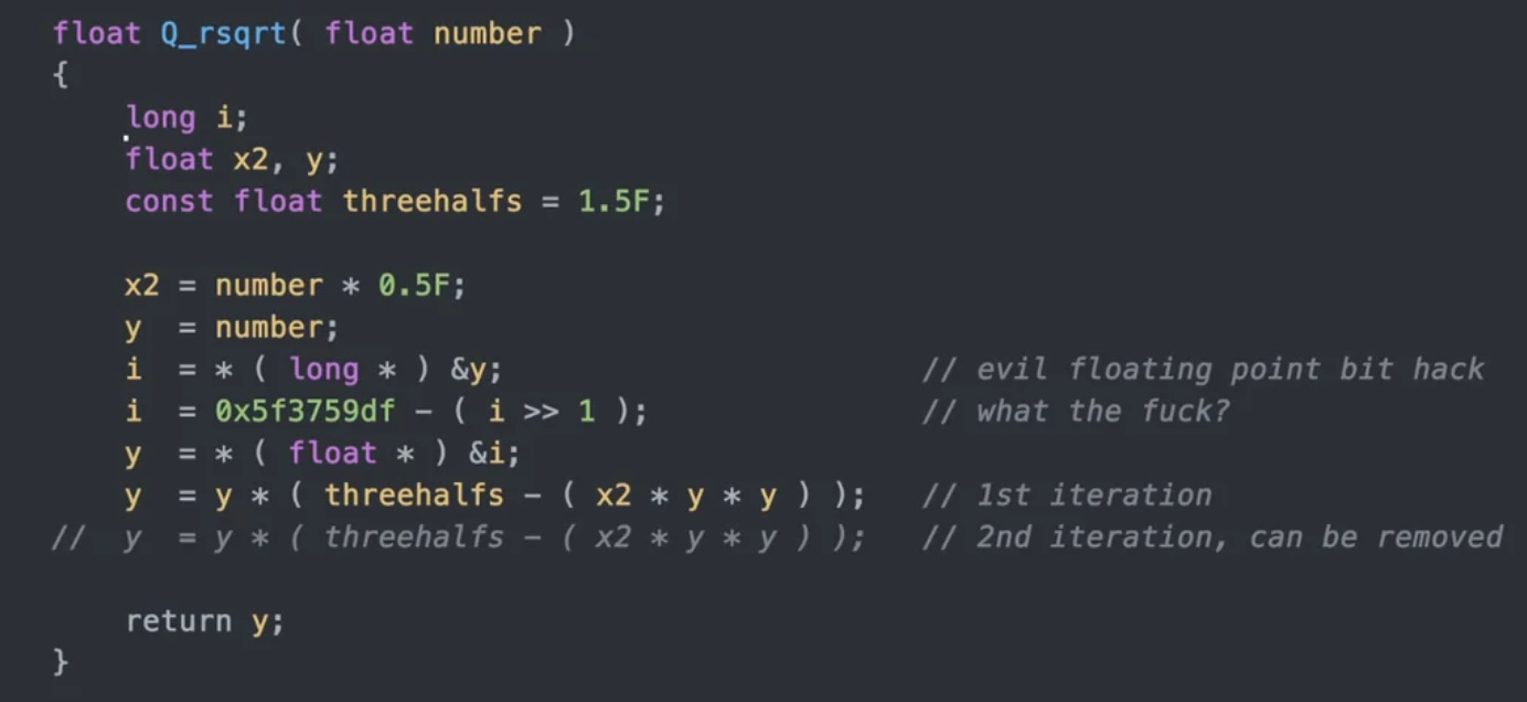
In the late 1980’s, software engineer Greg Walsh was working at Ardent Computer and had learned of a new algorithm. The algorithm had been outlined in a 1986 research paper, and was effectively a combination of computational bit-fiddling and applying Newton’s method to calculate inverse square roots very quickly. At the time it may have been an idea with some applications in numerical methods for computational physics (e.g. calculating things like inverse distances). Greg implemented and brought it to Ardent, but it didn’t immediately gain much traction.
It wasn’t until the late 1990’s, during the rise of computer gaming and 3D first person shooters like Doom and Wolfenstein that the algorithm found some real-world utility. Games with 3D graphics need to calculate parameters like angles of light incidence, distances to nearby objects, and reflections on surfaces many millions of times a second. In fact, this is exactly why we have GPU’s (graphical processing units) which are specialized computer chips to calculate these values in parallel and very quickly.
At the time, John Carmack was working at id Software on the graphics engine for Quake III. He found the fast inverse square root algorithm, which had meanderingly made its way to the company, and he implemented it in C. The algorithm had an immediate and significant improvement on the speed of the game’s graphic engine. Carmack had built an extremely high-leverage algorithm: a few lines of code that had a massive speed-up in running of the game. This is a kind of holy grail for engineers: finding these sorts of focal points, places where writing just a little code, or building a small tool can result in huge improvements in the rest of the system.
Routing Algorithms
Dijkstra’s algorithm is used to find minimum cost paths on graphs and serves as the basis of nearly all routing algorithms used for mapping services: Google uses Dijkstra’s as a basis to calculate shortest routes for its Maps products, faster variants of Dijkstra’s are used by Uber and Lyft to find the best drivers to service you, and companies like FedEx and UPS use routing algorithms to create optimized delivery schedules for their drivers. For the last 60 years, Dijkstra’s has been used as a basis for all modern routing algorithms in the transportation and logistics industry.
Earlier this year in April, researchers from Tsinghua University, Stanford, and the Max Planck School of Informatics published a paper outlining a new shortest-path algorithm that could deterministically improve upon Dijkstra’s algorithm for calculating shortest path distances, boasting a time complexity of O(m log2/3(n)) over Dijkstra’s O(m + n log(n))1. This is an asymptotic improvement to Dijkstra’s bound for sparse graphs (where the number of edges is comparable to the number of nodes) and interestingly enough, road networks can be modeled as graphs where the number of edges is roughly on order with the number of nodes.
It’s clear that an improvement upon Dijkstra’s algorithm could have not only an outsized impact on one company, but across an entire industry. So the question we’re left with is, have we finally found a routing algorithm that can overtake Dijkstra’s?
To answer this, we’re going to dive a little bit into how the algorithm works (I have a different post that really dives into the algorithm if you’re interested), what its limitations are, and whether this is going to be what CS students learn instead of Dijkstra’s.
Dijkstra’s Algorithm
Imagine you’re trying to find a route from your home to the grocery store that minimizes the ETA. If you knew how long it would take you to traverse each road segment, could you write a program to find the best route?
If you could transform your road network into a mathematical structure called a graph, you could use Dijkstra’s algorithm to find the shortest path from one node to another node. A graph, put simply, is a collection of nodes with edges that connect neighboring nodes (so in our example your home could be one node on the graph and the grocery store could be another). I find it helpful to draw graphs out, so here’s an example of a simple, weighted graph with numerical weights on the edges:
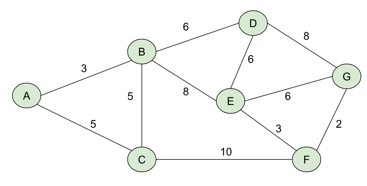
To find the least-cost path from A→G, we want to find a path (a sequence of nodes connected by edges), whose total weight is minimized over all possible paths from A→G. This is one of those mathematical statements that sounds a lot more complicated than it is. I’d encourage you to look at the graph above and see if you can find the least-cost path from A→G. Below I’ll outline it in blue:
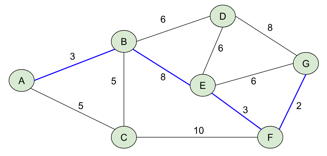
Hopefully you found this one (A→B→E→F→G), whose total weight is 3 + 8 + 3 + 2 = 16. I made this graph so that there was exactly one shortest path, but that’s not true in general (e.g. A→B→D→G and A→C→F→G are paths with weight 17).
In order to find this path, you may have tried a few options, backtracked when you realized there was something cheaper, etc. Dijkstra’s algorithm is just a formalized way of capturing this process in a set of rules you could write in a computer program.
Dijkstra’s works by keeping a sorted set of nodes to explore called a frontier. Once the frontier reaches the goal node, we can terminate the algorithm. In the graph above, we’d initialize our frontier with the starting node (A) and begin by exploring and the neighboring nodes (B and C) to our frontier, repeating the process until we reach the node of interest, G. There’s a little more bookkeeping in Dijkstra’s, (e.g. keeping track of the parent node, a cost map), but fundamentally the algorithm works by:
Exploring nodes in the frontier by picking the current “cheapest” node to expand from.
Keeping the frontier sorted via a priority queue data structure.
The second point is what leads to the computational bottleneck. In general, sorting a list of n elements scales with O(n log(n)) and there is no way to do better than this, generally speaking. In the case of routing, we require our frontier to be sorted, which means we will start to see computational bottlenecks as we use larger graphs.
So how does Google Maps provide routes from anywhere to pretty much anywhere? Improvements to routing have come not from using a completely new algorithm, but by reducing the size of the frontier, or number of nodes to search at any iteration. There are a number of ways to do this:
A*: A generalization of Dijkstra’s that uses heuristics to deprioritize obviously bad nodes during the search.
Contraction Hierarchies: Preprocesses the graph by running a lot of shortest path computations in advance, and then uses those computations to very quickly answer shortest path queries.
Multi-Level Dijkstra’s: Partitions the graph into multiple levels and preprocesses at the individual levels to parallelize the search across various levels.
Bidirectional Searches: Searches from the start and goal simultaneously and terminates when the frontiers of the searches “meet” around the middle.
Critically, each of these optimizations builds upon Dijkstra’s algorithm; in fact, the preprocessing pieces of each of these use Dijkstra’s as a kind of “first step” in calculating shortest paths.
Introducing BMSSP
As I mentioned, Dijkstra’s major bottleneck is that it must keep its searched nodes in sorted order to provide optimality guarantees, imposing a sorting barrier. For smaller problems this isn’t the worst thing in the world, but as problem instances grow, the need to sort the frontier of nodes becomes untenable.
In April, researchers Ran Duan, Jiayi Mao, Xiao Mao, Xinkai Shu, and Longhui Yin published Breaking the Sorting Barrier for Directed Single-Source Shortest Paths. The paper won a Best Paper Award at STOC for 2025 and claims to have broken the O(n log(n)) sorting barrier Dijkstra’s algorithm imposes on its frontier. Although the algorithm doesn’t have a specific name yet, it solves a variant of the shortest path problem called the “bounded multi source shortest path” (BMSSP). And so I’ll refer to it as such until we eventually come up with a better name for it.
What Dijkstra’s lacked in complexity, BMSSP has in spades. BMSSP is not an easy algorithm to follow, but the essential idea is based around continually shrinking the size of the exploration during the search, and avoiding having to sort too many nodes. The takeaway is that “breaking the sorting barrier” is based on intelligently selecting and removing nodes that we know won’t be important in later parts of the problem, and being able to deterministically do so, even for very large graphs.
BMSSP works by breaking down the shortest path problem into many “sub” problems. For example, BMSSP solves all of the shortest path costs to the closest set of nodes (without sorting them), and then seeds those nodes with initial distance estimates to solve.
The authors of the paper mention something a few times in their paper that I think is worth touching on:
“Dijkstra’s algorithm uses a frontier which is dynamic, and therefore intractable.”
What this means is that because Dijkstra’s holds the entire search frontier in memory, keeping it sorted, there’s no obvious way to partition the frontier without affecting optimality properties.
The BMSSP algorithm is clever in how it’s defined: it naturally contains a way to divide and conquer the shortest paths problem by breaking it up into bands, whereas Dijkstra’s doesn’t contain a natural means of dividing and conquering.
Divide and conquer is a very useful technique in software and can be illustrated nicely with sorting a list. For example, the gold-standard quicksort algorithm has a very simple, recursive solution. It selects an element as a pivot, divides up the list into to parts— one whose elements are less than the pivot and the other whose elements are greater. Then it runs quicksort again on those halves separately!
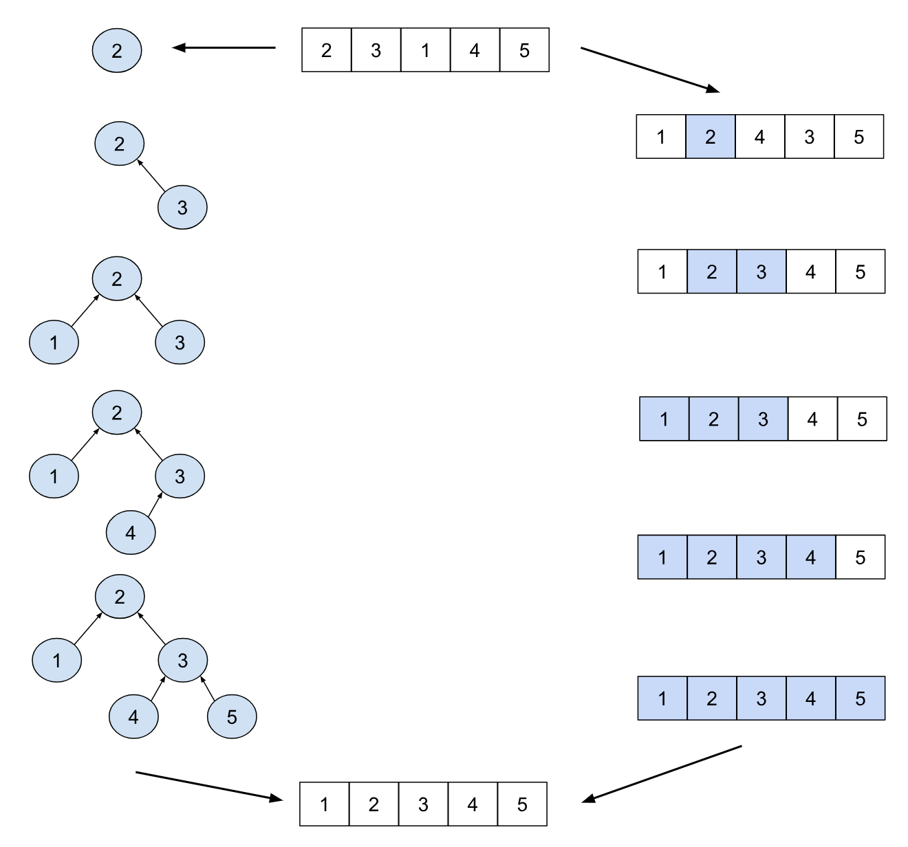
As a counterexample, consider the tree sort algorithm, which works by inserting elements into a binary search tree and then extracting them in order. The tree structure here is dynamic and can change as new elements are added in unpredictable ways, and doesn’t offer any immediate ways to parallelize like quicksort.
In addition to leveraging Divide-and-Conquer, BMSSP uses some other interesting techniques to cut down on its frontier size, such as finding pivot nodes that are necessary for the frontier to continue. This lets BMSSP search by expanding in “sections” from the beginning, identifying pivot nodes, and then shrinking the frontier down to those pivots recursively.
However, all of this overhead has a computational cost. BMSSP spends a lot of time in identifying pivot nodes and in determining when to stop expanding the frontier to “shrink” again. This means it won’t work better than Dijkstra’s for all graphs, but there might be some use cases where it will work really well (e.g. sparse graphs).
What Does it All Mean?
I’ve gone ahead and implemented the algorithm in Rust and currently the results are a little underwhelming: I’m seeing roughly a 5-6x slowdown in finding shortest paths using BMSSP compared to Dijkstra’s on large, road-network graphs. In the immediate term, I doubt this is going to be a huge lift. You’re not going to suddenly see faster routes on Google Maps and Uber isn’t going to start assigning you drivers more quickly. Keep in mind though, that the fast inverse square root algorithm took about 15 years to find a high leverage point in the industry and I think something similar could happen here.
It’s also worth noting that theoretical improvements like this don’t always translate well to the real world. For example, Dijkstra’s “official” time complexity is often cited as O(m + n log(n)), but this is if you implement it using an exotic priority queue called a Fibonacci heap. Fibonacci heaps are notoriously challenging to implement, and due to the way they’re structured they often don’t play well with how memory is laid out in computers. In practice, common implementations of Dijkstra’s use a binary heap, which technically bumps the time complexity up to O((m + n) log(n)), but they are usually much faster than Fibonacci heaps because they take advantage of CPU cache-locality and can be implemented without many recursive function calls.
There is reason to be hopeful though: it’s worth noting that my implementation is a non-memory optimized, faithful representation of the algorithm from the paper. It makes many not-so-optimal memory allocations and there is a ton of room for improvement. Modern implementations of BMSSP are the slowest they will ever be. If BMSSP can be implemented to be significantly faster than Dijkstra’s on road networks, I can see it being useful in a number of scenarios:
BMSSP+A*: BMSSP can naturally extend to using a heuristic and cut down on its frontier size even more by leveraging a smart heuristic like A*.
Matrix Calculations: For optimal dispatch problems, we need a large number of point-to-point ETAs calculated at once (e.g. every driver to every rider). If BMSSP speeds up, we could see these being calculated much more cheaply than they are today.
Preprocessing for Stronger Heuristics: Modern bidirectional A* implementations use landmark heuristics and reaches to preprocess road graphs while remaining flexible to cost changes. They often require solving many single source shortest paths problems, and BMSSP could be used instead of Dijkstra’s as a preprocessing tool.
Bidirectional BMSSP: I’m less certain about this one, but BMSSP might be able to be extended to bidirectional use cases (e.g. searching simultaneously from the origin and destination). Because BMSSP controls the bands of its frontier much better than Dijkstra’s, it might be able to converge faster, which would be a huge win.
I’ve included my BMSSP implementation here, where you can download and run the code if you’d like to mess around with it: I’d welcome any pull requests or changes if you see some obvious places for improvement! And if you’d like to learn more about the actual implementation and how the algorithm works in detail, check out my technical deep dive into BMSSP!
This is called “Big-O” notation in computer science and helps theorists describe asymptotic behaviors of algorithms as problem sizes grow. You can think of it like a rough mapping between the problem size and the time it takes to compute a solution. For example, O(N) means that the compute time grows linearly with the input size N (e.g. a problem 3 times larger will take 3 times as long to compute), but O(log(N)) would mean that a problem 10 times larger might only take twice as long to compute the solution (e.g. a binary search).